
Short answer
There is no fixed amount of training data that acoustic quality inspection needs. The requirement depends on the task (anomaly detection needs only normal data; classification needs examples of every defect), on how clearly defects change the sound, and on how much normal production varies. The reliable way to size it is a pilot recording and a learning curve on grouped data.
Key takeaways
- Count independent units such as parts, batches, tool states and recording sessions, not audio clips, because clips from the same part or session are strongly correlated.
- Anomaly detection can start with normal production data only, while defect classification needs enough confirmed examples of every defect class across the expected variation.
- The variability of normal production, such as product variants, tool wear and background noise, often drives the data requirement more than the defect itself.
- A learning curve on grouped validation folds shows whether more data will help and lets you extrapolate how much, instead of guessing.
- Public benchmarks such as MIMII and DCASE show typical research data set sizes, but they are not targets for your process.
How much training data acoustic quality inspection needs is usually the first question in an acoustic inspection project, often phrased as "how many recordings do you need?". The honest answer is that nobody can give a number without seeing the process. What we can give is the list of factors that determine the number, and a method to estimate it from a small pilot campaign rather than from a rule of thumb.
Why there is no magic number
Statements like "you need 1,000 examples per class" circulate widely. They are not wrong in every case, but they are not derived from anything about your process, and they hide the factors that actually matter.
Consider two acoustic inspection tasks. In the first, a defect produces a loud, distinct click on an otherwise quiet station. In the second, a defect changes the spectral balance of a weld sound by a small amount, on a line with three product variants and a press hammering next door. Both are "acoustic quality inspection". The second needs far more data, and more varied data, than the first. A fixed number would be too high for one and too low for the other.
What counts as a training example?
Before counting, decide what you are counting. A ten-second recording cut into a hundred overlapping windows does not give you a hundred independent examples. The windows share the part, the tool state, the sensor mounting, the background noise and the operator. A model can learn any of these.
The useful unit is the thing that varies independently in production:
- the part or weld, for per-part inspection;
- the batch or material lot, if material properties change the sound;
- the tool state, such as a fresh or worn electrode or cutter;
- the recording session, which bundles mounting, ambient noise and settings.
When someone says "we have 50,000 clips", the first follow-up question is how many parts, batches and sessions those clips come from. This is the same grouping logic we recommend in validating industrial AI models.
The factors that set the amount
| Factor | Needs less data when | Needs more data when |
|---|---|---|
| Task | Detecting deviation from normal | Naming several defect classes or grading severity |
| Effect size | The defect produces a strong, distinct acoustic change | The change is small relative to normal variation |
| Variability of normal | One product, stable tools, quiet surroundings | Several variants, tool wear, changing materials, background machines |
| Class similarity | Defect classes sound very different | Classes differ only in subtle spectral details |
| Measurement consistency | Fixed sensor position and settings | Sensor remounted, gain changed, position varies |
| Deployment scope | Same station as training | New stations, lines or plants |
| Feature design | Physically motivated features | Model must learn features from raw spectrograms |
Two factors deserve emphasis.
The task rung. Anomaly detection can be trained on normal production only. Classification needs confirmed examples of each defect, and severity grading needs examples across a range of severity. The distinctions are explained in the model ladder. Moving up a rung multiplies the labelling effort.
Variability of normal. A model must learn what normal sounds like across everything that legitimately varies. If you produce three variants with two tool states in two shifts, normal has at least a dozen faces. Each needs enough examples. In many projects this, not the defect, sets the data requirement.
What public benchmarks show
Public data sets show the scale researchers work at. They are useful reference points, not targets.
The MIMII data set for malfunctioning industrial machines covers valves, pumps, fans and slide rails, seven individual machines per type. According to the full paper, it contains 26,092 normal and 6,065 anomalous ten-second segments recorded at 16 kHz, mixed with factory noise at signal-to-noise ratios of 6 dB, 0 dB and -6 dB.
The DCASE 2024 challenge task on first-shot anomalous sound detection deliberately reduces the data. Each section of the development set provides 990 normal clips from a source domain and only ten normal clips from a target domain that differs in speed, load or noise, with 100 normal and 100 anomalous clips for testing. The challenge exists precisely because real deployments rarely have plenty of data for every operating condition.
Neither benchmark resembles a specific quality inspection task. Both show that anomaly detection research works with hundreds to thousands of normal clips per machine, and that performance under changed conditions is the hard part.
How to estimate training data for acoustic quality inspection
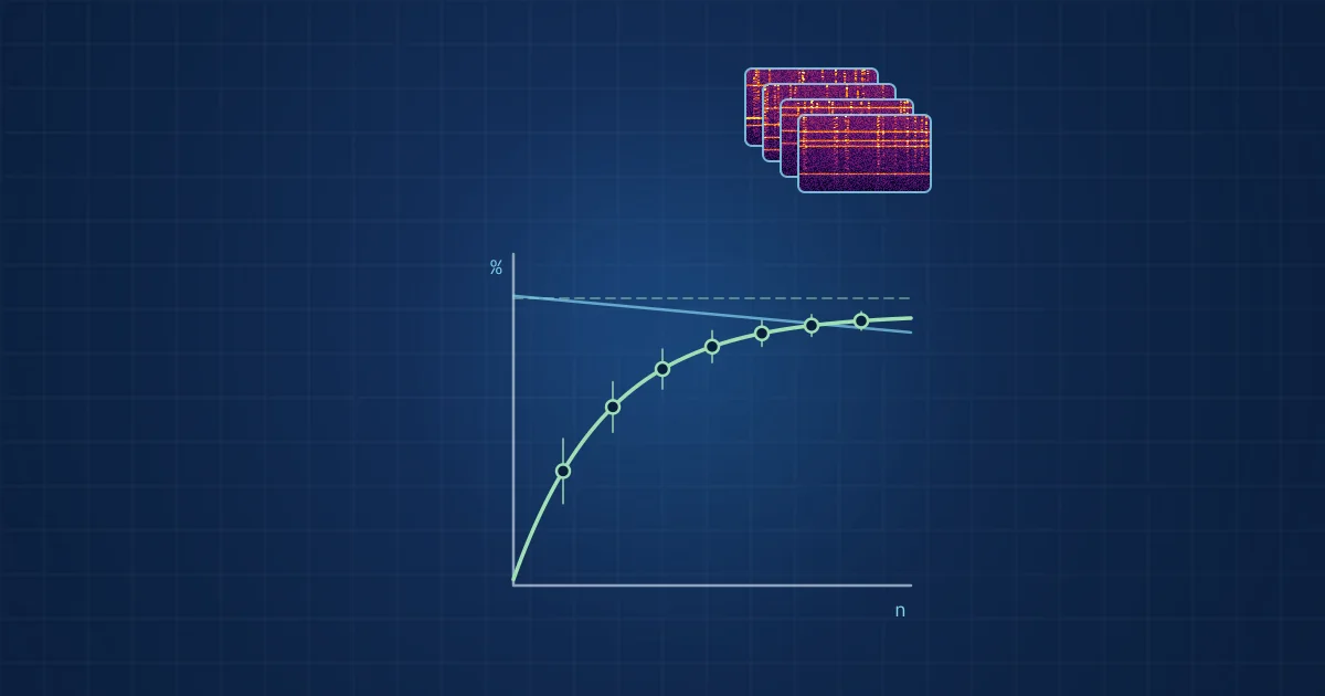
The most reliable estimate comes from your own data. A learning curve plots model performance against training set size. The scikit-learn documentation describes it as "a tool to find out how much we benefit from adding more training data and whether the estimator suffers more from a variance error or a bias error".
A procedure that works:
- Run a pilot campaign. Record a representative slice of production, covering the main variants, tool states and shifts, with good metadata. Include as many confirmed defects as you can obtain.
- Fix the grouping. Decide whether parts, batches or sessions are the independent unit. All validation splits respect it.
- Train at increasing sizes. Train the model on, for example, 10 %, 20 %, 40 %, 60 % and 80 % of the training groups, each time evaluating on held-out groups. Repeat with different group assignments to see the spread.
- Read the curve. If training and validation scores converge at a low value, the problem is bias: more of the same data will not help, and you need better features, a better sensor position or a different model. If a gap remains, more data is likely to help.
- Extrapolate carefully. Fitting an inverse power law to the learning curve gives a forecast of performance at larger sizes. Figueroa et al. (2012) studied this method for classification tasks and found that, depending on the data set, between 80 and 560 annotated samples were needed before the fitted curve predicted performance at larger sizes with low error. Treat the extrapolation as a planning estimate, not a guarantee.
- Plan the main campaign from the forecast, adding margin for conditions the pilot did not cover.
The output is a defensible answer: with this sensor, these features and this model, we expect to reach this performance with roughly this many parts or sessions, and here is the curve that says so.
Getting more from less data
Several techniques reduce the data requirement without pretending it away.
- Start with anomaly detection. It needs only normal data and can be used to find candidate defects for labelling.
- Use limit samples and seeded defects. Deliberately produced defects, made in agreement with quality engineering, fill gaps in rare classes. Check that they sound like real defects.
- Design features from physics. Physically motivated features need fewer examples than a network learning from raw spectrograms. See feature engineering for industrial signals.
- Fix the measurement. A rigid sensor mount, fixed gain and a consistent position remove variation the model would otherwise have to learn.
- Add a second modality. If sound alone cannot separate two defects, vibration or images may, which is often cheaper than collecting many more sound examples. We compare the two in acoustic vs vibration monitoring.
- Augment with care. Mixing in recorded background noise or shifting gain can help robustness. Synthetic defects are risky, because the model may learn the synthesis method.
A data collection checklist
- Independent units (parts, batches, sessions) are defined and logged.
- Every recording carries metadata: product variant, tool state, shift, sensor position and settings.
- Ground truth comes from an independent method, such as cross-sections, leak tests or end-of-line results.
- Normal production is recorded across all variants and conditions that will occur in deployment.
- Defect examples are spread across sessions, not concentrated in one test day.
- Background noise sources are documented and recorded both with and without defects.
- Raw audio is kept, not only features, so features can be recomputed later.
How NeuroControls approaches this
Our Acoustic Node uses a Microtech Gefell MK 301 E measurement capsule, with a 2 to 100 kHz capture band and production-proven use from 2 to 20 kHz. Recording that wide a band in pilot campaigns means the choice of analysis band can be made from data rather than fixed in advance. When the Acoustic Node is connected to the Edge AI Hub (built to order), recordings are stored with a versioned manifest and per-segment hashes, so pilot and main campaigns remain traceable.
Our engineers train custom models on customer data, from anomaly detection to classification and severity grading, as described on our models page. For weld inspection in battery production, our earlier e-WAS feasibility study recorded the vibro-acoustic response of each spot weld with a sensor integrated into the weld head, at 64 kSPS, and found that damping after a successful weld was clearly measurable and scaled with weld current, the kind of physical effect that keeps data requirements manageable.
Frequently asked questions
How many recordings do I need to train an acoustic inspection model?
There is no universal number. It depends on whether you need anomaly detection or defect classification, how strongly defects change the sound, how much normal production varies and how many conditions the model must cover. Run a pilot campaign, build a learning curve on grouped validation folds and extrapolate from it to plan the main data collection.
Can I train acoustic anomaly detection with normal data only?
Yes. Anomaly detection models learn what normal production sounds like and flag deviations, so they can be trained without defect examples. You still need some confirmed defects to check that the model actually reacts to them and to set a threshold. Normal data must cover all product variants, tool states and background conditions expected in operation.
Why do clips from the same recording not count as independent examples?
Clips cut from one recording share the same part, tool state, sensor mounting and background noise. A model can learn these shared characteristics instead of the defect, and a test set containing clips from the same recordings will overstate performance. Count parts, batches or recording sessions as the independent units when sizing and splitting data.
What is a learning curve and how does it help size training data?
A learning curve plots model performance against the amount of training data. If training and validation scores converge at a low value, more data will not help and you need better features or sensors. If a gap remains, more data is likely to help, and fitting a curve to the points gives a planning estimate of performance at larger sizes.
What sampling rate do I need for acoustic quality inspection?
It depends on where the defect's acoustic signature lies, and the sampling rate must be well above twice the highest frequency of interest. Friction, leaks and some process effects reach into the ultrasonic range, while others sit in the audible band. Recording a wide band in a pilot campaign lets you find the informative band from data before fixing the rate for production.
Sources and further reading
- Purohit et al. (2019): MIMII Dataset, sound dataset for malfunctioning industrial machine investigation and inspection
- DCASE 2024 Task 2: first-shot unsupervised anomalous sound detection for machine condition monitoring
- Figueroa et al. (2012): Predicting sample size required for classification performance, BMC Medical Informatics and Decision Making
- scikit-learn: validation curves and learning curves