
Short answer
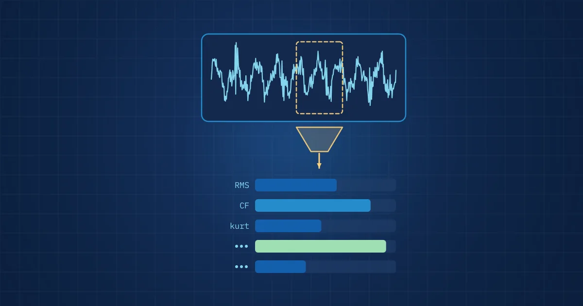
Feature engineering for industrial signals is the step that turns raw samples from accelerometers, microphones, cameras and thermal sensors into a compact set of numbers that describe the physical effect you care about. Good features start from the failure mechanism: which frequency band it excites, whether it is impulsive or tonal, and how it changes with speed and load.
Key takeaways
- Start feature engineering from the failure mechanism and its physical signature, not from the list of functions in a feature library.
- Time-domain features such as RMS, crest factor and kurtosis separate steady energy from impulsive events and are cheap enough for small edge processors.
- Envelope analysis exposes repetitive impacts, such as bearing defects, that are hidden under stronger low-frequency vibration in the raw spectrum.
- Normalising features for speed and load often matters more than adding new features, because operating conditions shift features as much as faults do.
- Compute normalisation statistics and feature selection on training data only, otherwise information from the test set leaks into the model.
Feature engineering for industrial signals decides most of what a model can and cannot learn. A classifier given RMS values alone will never see a bearing impact that barely changes the total energy. A classifier given a hundred loosely chosen features will find correlations that do not hold on the next machine. The work in between is less glamorous than model architecture and usually more decisive.
This article walks through how we build features for vibration, sound and thermal data, with enough detail to apply on your own data. It assumes you are familiar with the basics in vibration analysis from time signal to spectrum.
What is feature engineering for industrial signals?
A feature is a number, or a short vector, computed from a segment of raw signal that summarises a property of that segment. Feature engineering is the design of those computations so that the properties relevant to the task are preserved and irrelevant variation is suppressed.
Industrial signals make this harder than tabular business data for three reasons. They are high-rate, so a one-second vibration segment at 200 kSPS is 200,000 numbers. They are non-stationary, because machines change speed, load and temperature. And the interesting events are often small: a bearing defect in an early stage adds very little energy compared with the running vibration of the machine.
Start from the physics, not the library
The most productive question is not "which features exist?" but "what does this fault do to the signal?". Write it down for each failure mode before computing anything.
| Failure mechanism | What it does to the signal | Candidate features |
|---|---|---|
| Unbalance | Increases vibration at 1x running speed | Amplitude at 1x, RMS in low band |
| Misalignment | Raises 2x and sometimes 3x running speed, axial components | Ratios of 2x and 1x amplitudes, axial RMS |
| Rolling element bearing defect | Short periodic impacts that excite structural resonances | Kurtosis, crest factor, envelope spectrum at fault frequencies |
| Gear tooth damage | Modulation of the mesh frequency, sidebands | Sideband energy around mesh frequency |
| Leak or friction | Broadband high-frequency or ultrasonic noise | Band energy above several kHz, spectral flatness |
| Overheating contact | Local temperature rise relative to neighbours | Temperature difference to reference region |
This table is the start of a hypothesis, not a finished design. But it immediately tells you which sampling rate, which frequency band and which segment length you need. For bearings in particular, the expected impact frequencies follow from geometry, as explained in bearing fault frequencies explained.
Time-domain features
Time-domain features are computed directly on the sample values. They are cheap, robust and easy to explain to maintenance staff.
- RMS (root mean square): the square root of the mean of the squared samples. It measures overall signal energy and is the usual way to express broadband vibration magnitude, the quantity whose level and change over time are evaluated under ISO 20816-1, the general guideline for measuring and evaluating machine vibration.
- Peak and peak-to-peak: the largest excursion in the segment. Sensitive to impacts, but also to single spikes from electrical noise.
- Crest factor: peak divided by RMS. A pure sine wave has a crest factor of about 1.41. Impulsive signals have higher values, which is why crest factor rises in early bearing damage.
- Kurtosis: the fourth standardised moment, a measure of how heavy the tails of the amplitude distribution are. A Gaussian signal has a kurtosis of 3. Note that many libraries, including SciPy by default, report excess kurtosis, which is 0 for a Gaussian, so check the definition before setting thresholds. Repetitive impacts push it higher.
- Skewness: asymmetry of the amplitude distribution, useful for rubbing and one-sided clipping.
- Zero-crossing rate: how often the signal changes sign, a rough proxy for dominant frequency in acoustic data.
Crest factor and kurtosis have a known weakness: as bearing damage progresses and spreads, impacts become less distinct and both values can fall back towards normal. A feature that rises and then falls is useful for detection but misleading as a severity measure on its own. Combine it with energy-based features.
Frequency-domain and envelope features
Spectral features describe how energy is distributed over frequency. The usual starting point is a power spectral density estimate. SciPy's implementation of Welch's method does this by "dividing the data into overlapping segments, computing a modified periodogram for each segment" and averaging them, which trades frequency resolution for a smoother, more stable estimate.
From the spectrum, useful features include:
- Band energies: the integrated power in bands chosen from the physics table, for example around 1x and 2x running speed, around a gear mesh frequency, or in a high-frequency resonance band.
- Peak amplitudes at known frequencies: running speed harmonics, line frequency, blade pass frequency.
- Spectral centroid and spread: where the energy sits on average and how widely it is distributed.
- Spectral flatness: how noise-like a spectrum is. Leaks and friction tend to flatten it.
Envelope analysis deserves its own mention. A bearing defect produces short impacts that ring a structural resonance at a high frequency. In the raw spectrum this shows up as a broad hump, not as a line at the fault frequency. The remedy is to band-pass filter around the resonance, compute the amplitude envelope, then take the spectrum of the envelope. The SciPy documentation for the Hilbert transform states that "the amplitude envelope is given by the magnitude of the analytic signal". The envelope spectrum then shows lines at the impact repetition rate, which can be compared with the calculated bearing fault frequencies.
For acoustic data, mel-frequency cepstral coefficients (MFCCs) are a common default; librosa's implementation returns 20 coefficients unless told otherwise. Use them with care. The mel scale was designed around human pitch perception and compresses high frequencies, which is exactly where many machine faults and ultrasonic effects live. For industrial sound, linear band energies or a log spectrogram on a linear frequency axis are often the better starting point.
Segmentation, windowing and normalisation
How you cut the signal matters as much as what you compute.
Segment length should cover several periods of the slowest effect you care about. A segment of 0.1 s cannot resolve a modulation that repeats twice a second. For process monitoring, segmenting by process cycle (one weld, one press stroke) is usually better than fixed time windows, because each segment then corresponds to one part.
Operating conditions shift almost every feature. Vibration RMS rises with speed and load; acoustic levels change with feed rate; thermal readings depend on ambient temperature. Options to deal with this include:
- order tracking, which expresses frequencies as multiples of running speed rather than in hertz;
- normalising features per operating point, for example dividing by the median value observed at the same speed band during normal operation;
- including speed, load or ambient temperature as explicit inputs to the model.
Normalisation statistics must come from training data only. If you standardise features using the mean and standard deviation of the whole data set, including the test portion, the model gets a small but real hint about the test data. The same applies to feature selection: choosing the features that best separate classes on all data, then testing on a subset of that data, overstates performance.
Features from cameras, thermal and depth data
Vision models increasingly learn their own features, but engineered features remain valuable when data is scarce or the hardware is small.
- Thermal images: maximum, mean and percentile temperatures in regions of interest, and above all differences between regions. In an illustrative case, a motor terminal that is 15 K warmer than its neighbours says more than an absolute value that also depends on ambient temperature.
- Grey-scale images: intensity statistics in fixed regions, edge density, the area and position of bright or dark blobs.
- Depth data: distance statistics per zone, the change of a surface profile relative to a reference.
When several sensors observe the same event, combined features often carry the most information: the thermal rise in a region together with the vibration energy at the same time, or the acoustic signature of a weld together with the visual seam width. Our guide to multimodal sensing explains why.
A procedure for building a feature set
- List failure modes you need to detect, with their expected effect on each signal.
- Check acquisition: sampling rate at least a few times above the highest frequency of interest, sensor bandwidth and mounting adequate for that band.
- Define segments: fixed windows with overlap for continuous machines, cycle-based segments for processes.
- Compute a small baseline set: RMS, peak, crest factor, kurtosis and three to six band energies chosen from the physics.
- Plot before modelling: feature against time, against speed and load, and by class. Many problems, including mislabelled data and sensor faults, are visible here.
- Normalise for operating conditions, using statistics from training data only.
- Add targeted features (envelope spectrum lines, sidebands, region differences) where the baseline set does not separate the classes.
- Validate on held-out machines, batches or days, not on random segments from the same recording.
Automated tools such as tsfresh, described in its documentation as a tool "for systematic feature engineering from time-series and other sequential data", can generate hundreds of candidate features. They are useful for exploration. The more features you generate, though, the more important step 8 becomes, because some of them will separate your training data by chance.
Engineered features or learned features?
Deep networks on spectrograms or raw waveforms can learn features directly and sometimes outperform hand-crafted sets, especially on complex image defects. They also need more data, more compute and more careful validation, and their features are harder to explain to the engineer who has to act on an alarm.
On constrained edge hardware, a common compromise is to use engineered features for continuous monitoring and reserve learned models for events, such as a short segment around a detected anomaly. The edge context is explained in what is edge AI in manufacturing, and the next step, turning features into anomaly scores, classes and grades, in the model ladder.
How NeuroControls approaches this
Feature extraction is part of every custom model we build: our engineers train models on customer data, with feature extraction, anomaly detection, classification and severity grading as separate, testable stages. The approach is described on our models page.
Because features are only as good as the recordings behind them, our software records raw data on site with a versioned manifest and exports to open formats such as NWB, JSONL and CSV, so features can be recomputed when a better definition is found.
Frequently asked questions
What is feature engineering in condition monitoring?
It is the design of calculations that turn raw sensor samples into numbers describing machine condition, such as RMS, kurtosis, band energies or envelope spectrum amplitudes. Good features are chosen from the failure mechanisms you expect, so that each one responds to a physical effect like an impact, an imbalance or a temperature rise, and ignores irrelevant variation.
Which vibration features are most useful for machine learning?
A robust starting set is RMS, peak, crest factor, kurtosis and a handful of band energies chosen around running speed harmonics and structural resonances. For bearings, add envelope spectrum amplitudes at the calculated fault frequencies. Normalise these for speed and load, then add more targeted features only where the baseline set fails to separate the classes.
Why is kurtosis used for bearing fault detection?
Kurtosis measures how heavy the tails of a signal's amplitude distribution are. A Gaussian signal has a kurtosis of 3, while repetitive impacts from a damaged bearing raise it. It is sensitive in early damage stages, but it can fall again as damage spreads and impacts become less distinct, so it should not be used alone for severity.
Should I use MFCCs for machine sound analysis?
MFCCs are a reasonable baseline but not always the best choice. The mel scale is based on human pitch perception and compresses high frequencies, where many machine faults, leaks and friction effects have their energy. Linear band energies or a log spectrogram on a linear frequency axis often preserve more of the relevant information for industrial sound.
How do I avoid data leakage in feature engineering?
Compute normalisation statistics, feature selection and any other data-dependent step on training data only, then apply the fixed transformations to the test data. Split test data by machine, batch or time period rather than randomly by segment, because segments from the same recording share characteristics that a model can memorise.