
Short answer
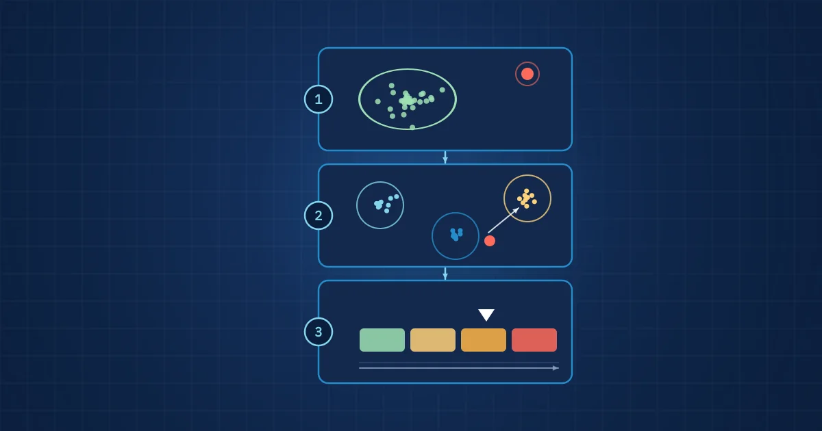
Anomaly detection, classification and severity grading answer three different questions. Anomaly detection asks whether a signal differs from normal and can be trained on normal data alone. Classification asks which known fault it is and needs labelled examples of each fault. Severity grading asks how bad it is and needs examples across a fault's progression or a defined physical scale.
Key takeaways
- Anomaly detection, classification and severity grading are separate model types with different data requirements, not settings of one model.
- Anomaly detection is usually the first rung because it can be trained on normal operation only, but it cannot say what is wrong.
- A fault classifier only knows the classes it was trained on, so it should run behind an anomaly gate that catches conditions it has never seen.
- Severity grading is an ordinal problem: grades must be ordered, monotonic and tied to an action, not just treated as more classes.
- Thresholds for each rung should be set on held-out data from the plant, in terms operators understand, such as false alarms per week.
Anomaly detection, classification and severity grading are often lumped together as "AI for condition monitoring", as if one model could do all three. In practice they are three rungs of a ladder. Each answers a narrower question than the one below it and needs more specific data. Knowing which rung you are on, and which one you can realistically reach with the data you have, saves months on industrial AI projects.
This article explains each rung, how they fit together at runtime, and where each typically fails. It builds on feature engineering for industrial signals, because all three rungs depend on good inputs.
Three questions, three model types
The ladder has three rungs:
- Is this normal? Anomaly detection.
- What is it? Classification.
- How bad is it, and what should we do? Severity grading.
The same structure appears in ISO 13374, the series on data processing for condition monitoring. Its data-processing part lists separate blocks for state detection, health assessment, prognostic assessment and advisory generation, as shown in the ISO 13374-2 table of contents. State detection corresponds roughly to the first rung, health assessment to the second and third. Separating the questions is not an AI invention; it is how condition monitoring has been organised for decades.
Rung 1: anomaly detection
Anomaly detection is the identification of observations that do not fit the pattern of normal data. In industrial use, the variant that matters most is what the scikit-learn documentation calls novelty detection: the training data "is not polluted by outliers and we are interested in detecting whether a new observation is an outlier". You train on normal operation and ask whether new data looks like it.
That property is the main reason anomaly detection is the first rung. At the start of a project you rarely have recorded faults, but you can usually record weeks of normal running.
Common methods include:
- Distance and density methods, such as Mahalanobis distance on a feature vector or local outlier factor, which flag points far from the bulk of normal data.
- Isolation forests, which isolate points with random splits; anomalies need fewer splits.
- One-class support vector machines, which learn a boundary around normal data.
- Autoencoders, neural networks trained to reconstruct normal inputs; a high reconstruction error suggests something new.
The output is a score, not a decision. Turning it into an alarm needs a threshold, and that threshold should be set on held-out normal data from the real installation. Express it in operational terms: at this threshold, how many alarms per week would normal operation produce? An anomaly detector with a nominal false positive rate of 1 % sounds good until you calculate that it evaluates a segment every second. That is 864 false alarms a day, about 6,000 a week, if segments are independent.
What anomaly detection cannot do is tell you what changed. A new product variant, a maintenance intervention, a different shift pattern and a developing bearing fault all look "abnormal". That is useful, because it shows the operating envelope has moved, but it is not a diagnosis.
Rung 2: fault classification
Fault classification assigns a signal to one of a set of known classes: normal, unbalance, misalignment, outer race defect, cavitation, and so on. In quality inspection the classes are defect types: porosity, spatter, lack of fusion, misalignment of a part.
Classification needs labelled examples of every class. That is the hard part. Faults are rare on healthy plants, and labels come from maintenance records, teardown findings or lab analysis that are slow and expensive. Common sources of training data are test rigs with seeded faults, historical recordings with confirmed maintenance findings, and inspected reject parts.
Three issues come up again and again:
- Closed-set assumption. A classifier always picks one of the classes it knows. Show it a fault type it has never seen and it will confidently name the closest known one. Running classification only on segments that the anomaly detector has flagged, and reporting "unknown anomaly" when the classifier's confidence is low, keeps this under control.
- Multiple simultaneous faults. Real machines can have misalignment and a bearing defect at the same time. A single-label classifier must choose; a multi-label classifier can report both. If combined faults are plausible, design for multi-label output from the start.
- Class imbalance. With thousands of normal examples and a few dozen faulty ones, accuracy is a misleading metric. Report per-class recall and precision, and look at the confusion matrix.
Physically similar faults are hard to separate with a single sensor. Different sensing modalities often disambiguate them, which is the argument in why single-sensor monitoring misses faults.
Rung 3: severity grading
Severity grading assigns an ordered grade to a detected condition, for example "minor", "monitor closely", "plan intervention", "act now". It is the rung that operators actually need, because it connects a finding to an action.
It is also the most misunderstood rung. Severity grades are not just more classes. They are ordinal: grade 3 is worse than grade 2, which is worse than grade 1. A good grading model respects that order, so that a slowly worsening fault moves up the scale step by step instead of jumping between grades.
There are three ways to define the scale:
- Standard-based scales. For overall vibration, ISO 20816-3 evaluates broadband vibration of industrial machines above 15 kW against evaluation zones. Where a standard exists, use it as a reference grade. Our article on ISO 20816 vibration severity zones covers what the zones mean in practice.
- Physics-based scales. Defect size, wear depth, crack length or weld penetration measured on inspected parts. These require teardown or lab measurements, but give grades a physical meaning.
- Consequence-based scales. Grades defined by the required action and its urgency, agreed with maintenance or quality staff.
Severity grading also needs probability outputs you can trust. A model that says "80 % grade 3" should be right about 80 % of the time when it says so. The scikit-learn guide on probability calibration explains the concept and two standard correction methods, sigmoid (Platt) scaling and isotonic regression. Calibrated probabilities make it possible to set grade thresholds deliberately rather than by trial and error.
Finally, grades should be smoothed over time. A single segment rarely justifies an escalation; a grade that persists over many segments or operating cycles does.
Anomaly detection, classification and severity grading at a glance
| Anomaly detection | Classification | Severity grading | |
|---|---|---|---|
| Question | Is this different from normal? | Which known fault or defect is it? | How bad is it, and what action follows? |
| Training data | Normal operation only | Labelled examples of every class | Examples across fault progression, or a defined physical scale |
| Typical methods | Isolation forest, one-class SVM, autoencoder, distance to normal | Gradient-boosted trees, neural networks, multi-label classifiers | Ordinal regression, calibrated classifiers, trend models |
| Output | Score and threshold | Class label with confidence | Ordered grade with confidence |
| Typical failure | Alarms on harmless changes in operation | Confidently names the wrong known class for an unseen fault | Grades jump around or do not match the required action |
How the rungs work together at runtime
In a deployed system the three models run as a chain, each gating the next:
- Features are computed for every segment or process cycle.
- The sensor health check confirms the input is valid. A loose sensor should never reach the fault models.
- The anomaly detector scores the segment. Below threshold, the segment is recorded as normal.
- Above threshold, the classifier assigns a fault class or reports "unknown anomaly" if confidence is low.
- For a known class, the severity model assigns a grade.
- Temporal logic confirms the grade over several segments before raising or escalating an alert.
- The result is stored with the model versions and the evidence (features and raw segment) that produced it.
Step 2 is often forgotten, and we return to it in our article on self-monitoring sensors. Step 7 is what makes the chain auditable and improvable: every confirmed or rejected alert becomes a labelled example for the next training round.
Where to start
Before choosing a rung, decide which failure modes matter. ISO 17359, the general guideline for condition monitoring programmes, puts a reliability and criticality audit, including failure modes, effects and criticality analysis, ahead of the choice of monitoring method. The same order works for models. Then use this checklist to decide which rung to build first:
- Only normal data available? Start with anomaly detection and use it to collect and label the first abnormal events.
- Seeded-fault rig or confirmed historical faults available? Build a classifier, but keep the anomaly detector in front of it.
- Inspected parts or teardown measurements available? You can define a physics-based severity scale.
- Maintenance team agrees on actions per grade? You can define a consequence-based scale and grade against it.
- None of the above? Invest in recording first. A good data set outlives any model.
Whatever the rung, validate on data from machines, batches or time periods the model has not seen. Random splits of segments from the same recordings overstate performance, a point we cover in detail in validating industrial AI models. The overall context is in what is edge AI in manufacturing.
How NeuroControls approaches this
Our engineers train custom models on customer data along exactly this ladder: feature extraction, anomaly detection, fault and multi-fault classification, and severity grading. On-device inference as ONNX on the node CPU was first proven on our Vibration Node; NPU deployment is coming soon. Details are on our models page and, for machine monitoring use cases, on our condition monitoring solutions page.
Each sensor in our systems reports its signal health and dropouts alongside the data, so a gap in the data is flagged in the record.
Frequently asked questions
What is the difference between anomaly detection and fault classification?
Anomaly detection asks whether new data differs from normal operation and can be trained on normal data alone. Fault classification asks which known fault is present and needs labelled examples of each fault type. Anomaly detection finds the unexpected but cannot name it; classification names faults but only those it was trained on, so the two are usually combined.
What is severity grading in condition monitoring?
Severity grading assigns an ordered grade to a detected condition, such as minor, monitor, plan intervention or act now. The scale can follow a standard, a physical measure like defect size, or agreed maintenance actions. Unlike plain classification, grades are ordinal, so a good model moves a slowly worsening fault up the scale step by step.
Can anomaly detection be trained without fault data?
Yes. Novelty detection methods such as isolation forests, one-class support vector machines and autoencoders are trained on normal operation only and flag data that does not fit. This is why anomaly detection is usually the first model on a new machine. The detected anomalies can then be inspected and labelled to build training data for classification.
How do you set an anomaly detection threshold?
Set it on held-out normal data from the real installation and express it in operational terms, such as expected false alarms per week. Then check how quickly known or seeded faults cross it. A small percentage false positive rate can still mean many alarms per day if the model evaluates a segment every second, so always convert rates into counts.
Why should a fault classifier run behind an anomaly detector?
A classifier always chooses one of the classes it knows, even for a fault it has never seen. Running it only on segments the anomaly detector has flagged, and reporting an unknown anomaly when classifier confidence is low, prevents confident but wrong diagnoses. It also reduces computation, because the classifier only runs when something unusual has happened.