
Short answer
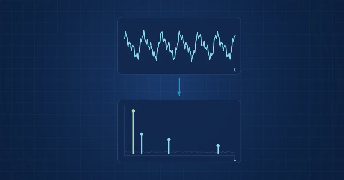
Vibration analysis turns an accelerometer's time signal into a frequency spectrum, usually with a fast Fourier transform (FFT). The time signal shows how much the machine moves; the spectrum shows at which frequencies, which links energy to shaft speed, gear meshes, bearings or resonances. Getting it right depends on four choices: sample rate, record length, window and averaging.
Key takeaways
- The sample rate sets the highest frequency you can trust, and must comfortably exceed twice that frequency because of anti-aliasing filter roll-off.
- Frequency resolution equals the sample rate divided by the number of samples, so separating close peaks needs a longer record, not a faster sample rate.
- A Hann window is the right default for machine vibration; a flat-top window is for reading the amplitude of a single tone accurately.
- Overall vibration level tells you whether something changed; the spectrum tells you what changed.
Vibration analysis basics come down to one idea: a machine's vibration is a sum of periodic and random components, and the spectrum separates them by frequency. An accelerometer on a bearing housing records a time signal, a few seconds of acceleration values. On its own that signal is hard to read. Converted into a spectrum, it becomes a list of frequencies with amplitudes, and many of those frequencies have mechanical names.
This post walks through that conversion step by step, from the sensor to a spectrum you can defend in a maintenance meeting. It is written for engineers who know what a bearing is but have not set up an FFT analyser themselves.
What the time signal already tells you
The time waveform is the raw record: acceleration sampled at fixed intervals. Before any transform, a few statistics already carry useful information. They are cheap to compute and they are the first features most monitoring systems track.
| Time-domain metric | What it is | What it is good for |
|---|---|---|
| RMS | Root mean square of the signal, the energy-related average level | Trending overall condition; basis of most severity limits |
| Peak | Largest absolute value in the record | Spotting impacts and shocks |
| Crest factor | Peak divided by RMS | Early impacting from local defects, before RMS rises |
| Kurtosis | Fourth standardised moment, "peakiness" of the distribution | Short repetitive impulses, typical of early bearing damage |
The limitation is obvious once you think about it. RMS rises for unbalance, for looseness, for a damaged bearing and for a neighbouring machine that has just started. It says that something changed, not what. For that you need frequency.
From time signal to spectrum: the FFT in plain terms
For a real signal, the discrete Fourier transform of a block of N samples gives N/2 + 1 frequency lines from 0 Hz to Nyquist; analysers typically display about N/2.56 of them, because the top of the band sits inside the anti-aliasing filter's roll-off. The FFT is simply a fast algorithm for computing the transform. Each line represents a narrow frequency band, and its height shows how much of the signal's energy sits there.
Three relationships define what the spectrum can show:
- Maximum frequency. The Nyquist frequency is half the sample rate. Anything above it folds back into the spectrum as a false peak, which is called aliasing. An analogue anti-aliasing filter must remove it before the converter, and because no filter is perfectly sharp, the usable range ends some way below Nyquist.
- Resolution. The line spacing is the sample rate divided by N, which is the same as one divided by the record length in seconds. A 1-second record gives 1 Hz lines; a 4-second record gives 0.25 Hz lines.
- Trade-off. Doubling the sample rate without doubling N doubles the frequency range and doubles the line spacing, so the resolution becomes twice as coarse. Fine resolution at high frequency needs long records and therefore more data.
A short example makes this concrete. A four-pole motor running at 1,480 rpm turns at about 24.7 Hz. Suppose a neighbouring fan on a different drive runs at 1,500 rpm, or 25.0 Hz, and its vibration reaches your sensor through the frame. The two peaks are about 0.3 Hz apart. A windowed peak spreads over several lines, so you want a line spacing of roughly 0.1 Hz, which means a record of about ten seconds. A one-second capture would merge them into one peak and you would blame the motor for the fan.
Windowing: why the edges of the record matter
The FFT assumes the record repeats forever. If the signal does not contain a whole number of cycles, the end of the record does not join its start, and that discontinuity smears energy across neighbouring lines. This is spectral leakage. As National Instruments puts it in its note on FFTs and windowing, when the number of periods in the acquisition is not an integer, the endpoints are discontinuous.
A window function tapers the record towards zero at both ends to reduce that smearing. The choice matters less than people think, but it does matter:
- Hann (Hanning) is the general-purpose choice for machine vibration. The same NI note says it is satisfactory in 95 percent of cases.
- Flat top gives the most accurate amplitude for a single tone, at the cost of wider peaks. Use it when calibrating or when an amplitude figure is the deliverable.
- Uniform (no window) suits broadband random signals and transient captures that start and end at zero.
Whatever you choose, write it down. Two spectra with different windows are not directly comparable in amplitude.
Units: acceleration, velocity and displacement
Accelerometers measure acceleration, but vibration is often discussed in velocity or displacement. The three are related by integration, and each one emphasises a different part of the spectrum. Acceleration grows with frequency for the same displacement, so it highlights bearing and gear-mesh content in the kilohertz range. Displacement is dominated by low frequencies, which suits shaft movement in sleeve bearings.
Velocity sits in between and is the usual unit for overall machine condition. Severity guidelines such as ISO 20816-1:2016 evaluate machines on broadband vibration magnitude and on changes in that magnitude, which is why a velocity trend is the first thing most maintenance teams look at. We cover the severity zones themselves in our post on ISO 20816 zones A to D.
One caution on integration: integrating acceleration amplifies low-frequency noise. Most analysers apply a high-pass filter first, often at a few hertz. If a velocity spectrum shows a large ramp towards 0 Hz, that is almost always an integration artefact, not a machine fault.
A practical procedure: from sensor to spectrum
This is the sequence we use when setting up a new measurement point. It is deliberately boring, because spectra go wrong in boring ways.
- Define the fault frequencies you care about. List shaft speeds, gear meshes, blade-pass frequencies and bearing defect frequencies. Our article on bearing fault frequencies shows how to calculate the last group.
- Choose the sensor and its mounting. Check the accelerometer's usable band against your highest frequency of interest. A MEMS sensor such as the Analog Devices ADXL1002 is specified at plus or minus 50 g with a 3 dB bandwidth up to 11 kHz (within 5 % up to 4.7 kHz) and a resonance around 21 kHz. Stud or adhesive mounting keeps the mounted resonance high; a magnet lowers it.
- Set the sample rate. Make it well above twice the highest frequency of interest so the anti-aliasing filter has room to roll off.
- Set the record length. Pick N so that the line spacing resolves the closest pair of frequencies you need to separate, for example running speed and its sidebands.
- Apply a window. Hann, unless you have a specific reason.
- Average. Average several spectra, with 50 percent overlap if the analyser supports it, to reduce random noise. Linear averaging of the power spectrum is the default for stationary machines.
- Record the operating state. Speed, load and temperature at the time of capture. A spectrum without operating context cannot be compared with next month's.
- Compare against a baseline. Store the first good spectrum per point and operating state, and judge changes relative to it.
The standard that covers this processing chain in detail is ISO 13373-2:2016, which deals with processing, analysis and presentation of vibration data, including time-domain and frequency-domain analysis and signal enhancement.
Reading a spectrum without fooling yourself
Once the spectrum is clean, interpretation starts with orders: frequencies expressed as multiples of running speed. A peak at 1x running speed often points to unbalance. Strong 2x and axial components are a common sign of misalignment. Many harmonics of running speed with a raised noise floor suggest mechanical looseness. These are heuristics, not rules, and every experienced analyst has a story about a 2x peak that turned out to be something else.
Non-synchronous peaks, those that are not integer multiples of running speed, deserve the most attention. Bearing defect frequencies are non-synchronous by design. So are electrical frequencies tied to line supply, and resonances excited by broadband impacts.
Checklist of common mistakes:
- Comparing spectra taken at different speeds without converting to orders.
- Reading amplitude from a Hann-windowed spectrum as if it were a calibrated tone.
- Treating an aliased peak as real because the anti-aliasing filter was disabled.
- Mounting the sensor on a thin cover plate that has its own resonance.
- Forgetting that a loose or failing sensor also changes the spectrum.
The last point is underrated. A sensor that has partly detached produces a spectrum that can look like looseness in the machine. That is why the sensor itself has to be checked before the spectrum is read, a theme we return to in what multimodal sensing is and why it helps.
How NeuroControls approaches this
Our Vibration Node digitises a single channel at 18 bits and 200 kSPS through an ADAQ4003 converter, with an LTC6373 programmable-gain amplifier ahead of it and an ADI ADXL1002 accelerometer. That gives generous headroom above the sensor's band, so the anti-aliasing filter can do its job without eating into the frequencies that matter. Every stream is time-stamped on the hub, and the node flags signal health and dropouts with every segment, so a gap is visible in the record.
Spectra and time-domain features feed the models our engineers train on customer data, from anomaly detection to fault classification and severity grading. The Machine Health Kit combines the Vibration Node with an Acoustic Node on one hub, and the condition monitoring solution page describes how the pieces fit together. If you are planning a first measurement campaign, our notes on models and validation are a good next read.
Frequently asked questions
What sample rate do I need for vibration analysis?
The sample rate must be more than twice the highest frequency you want to analyse, because of the Nyquist limit, and in practice clearly higher so the anti-aliasing filter can roll off before Nyquist. For running-speed faults a few kilohertz is enough. For bearing and gear-mesh analysis, which reaches into the kilohertz range, sample rates of tens of kilohertz or more are common.
How do I improve frequency resolution in an FFT?
Frequency resolution equals the sample rate divided by the number of samples, which is the same as one divided by the record length in seconds. To get finer resolution you must record for longer, or lower the sample rate if the frequency range allows it. Zero padding makes the plot smoother but does not separate peaks that the record length cannot resolve.
Which FFT window should I use for vibration data?
Use a Hann window as the default for machine vibration, because it controls spectral leakage well for most signals. Switch to a flat-top window when the accurate amplitude of a single tone is what you need, for example during calibration. Use no window for transients that start and end at zero. Always record the window, because it changes amplitude readings.
Should I analyse vibration in acceleration or velocity?
Both, for different purposes. Velocity is the usual unit for overall machine condition and is what most severity guidelines are built around. Acceleration emphasises high frequencies, so it is better for early bearing and gear defects. Displacement suits low-frequency shaft motion. Many analysts trend overall velocity and inspect acceleration spectra and envelopes for detail.
Why does my velocity spectrum rise sharply near 0 Hz?
That ramp is usually an integration artefact. Converting acceleration to velocity divides each line by 2 x pi x f, the angular frequency, which amplifies low-frequency noise and sensor drift. Analysers normally apply a high-pass filter before integration to suppress it. If the ramp persists, check the filter setting and the sensor's low-frequency specification before suspecting the machine.
Sources and further reading
- National Instruments: Understanding FFTs and Windowing
- ISO 20816-1:2016 Mechanical vibration - Measurement and evaluation of machine vibration - Part 1: General guidelines
- ISO 13373-2:2016 Vibration condition monitoring - Part 2: Processing, analysis and presentation of vibration data
- Analog Devices ADXL1002 product page
- Analog Devices ADAQ4003 product page